The following tools make it easy to analyze these NRES spectra. Students can investigate the spectra of single stars, binary star systems, and even highly variable stars without needing advanced experience.
Topics include:
- Feel the Earth’s Movement through Space
- Spectral Analysis and Stellar Classification
- The Dynamics of Binary Star Systems
- Variable and Unstable Stars
- Research Projects and Advanced Astronomy Activities
TOOL 1: NRES Data Analyzer
mail@tobiasbreitenstein.de
The "Spectral Lines" and "Goto Line" menus can be customized with external files. You can place a marker anywhere in the spectrum by left-clicking.
Keyboard Controls
- Right/Left Arrow Keys - move through the spectrum
- +/- Key - zoom in or out along the wavelength axis
- Up/Down Arrow Keys - adjust the flux scale
- Click and V - calculate the Doppler Velocity using the nearest spectral line
- Click and C - calibrate the spectrum to the nearest spectral line (for example, to correct for Doppler shifts)
- Click and N - search the NIST Database by selected wavelength +/- 0.01 nm (calibrate spectrum first!)
- Click and M - measure distance between two points
TOOL 2: NRES Data Extractor
The NRES Data Extractor converts data from "...-e92-1d.fits.fz" files into CSV files. These files can then be explored and analyzed using spreadsheet software such as Excel, LibreOffice Calc, and Google Sheets or a Python program.
Caution: Please extract only small sections of a spectrum, such as individual spectral lines. Large exports can contain a huge amount of data and may slow down or overload your browser.
To avoid this issue, only an image and a link to the tool are provided here: NRES Data Extractor
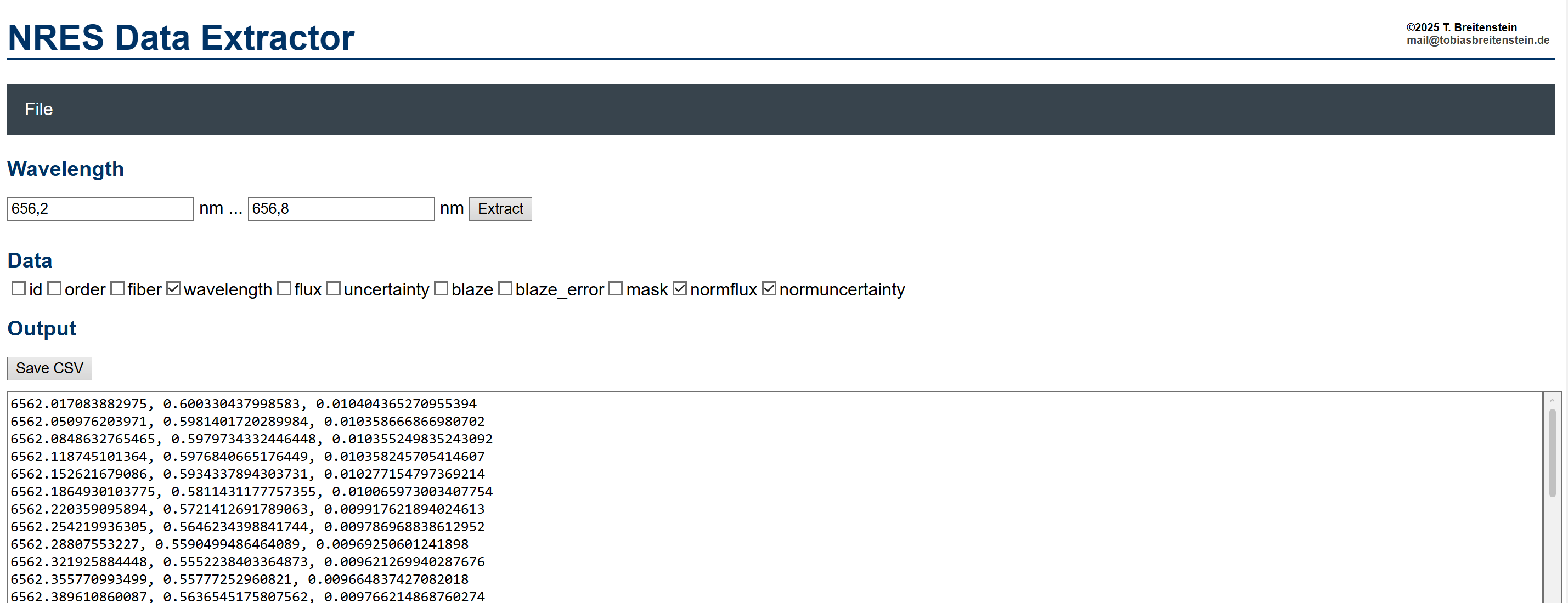
The main purpose of the NRES Data Extractor is to support a more detailed investigation of individual spectral lines and their shapes. For examples of how this can be done, see Examples 3, 4a, 4b, and 5 at the bottom of this page.
Application Examples & Demonstrations
Using Rigil (Alpha Centauri), this animation shows how the Hα line of a star appears to shift back and forth over the course of a year because Earth is orbiting the Sun.
When Earth moves toward the star, the spectral line shifts slightly toward shorter wavelengths (blueshift). When Earth moves away from the star, the line shifts toward longer wavelengths (redshift). This effect is known as the Doppler effect.
When the star’s measured radial velocity (its speed toward or away from Earth) is plotted against the observation date, the result is a sine wave with a period of about 365.25 days, caused by Earth’s motion around the Sun.
If the star itself is also moving through space, the entire curve may shift upward or downward. This shift provides information about the star’s velocity relative to our solar system.
While the star's Hα line shifts over the course of the year due to the Doppler effect, the lines of Earth's atmosphere like oxygen (O2) stay in the same position.
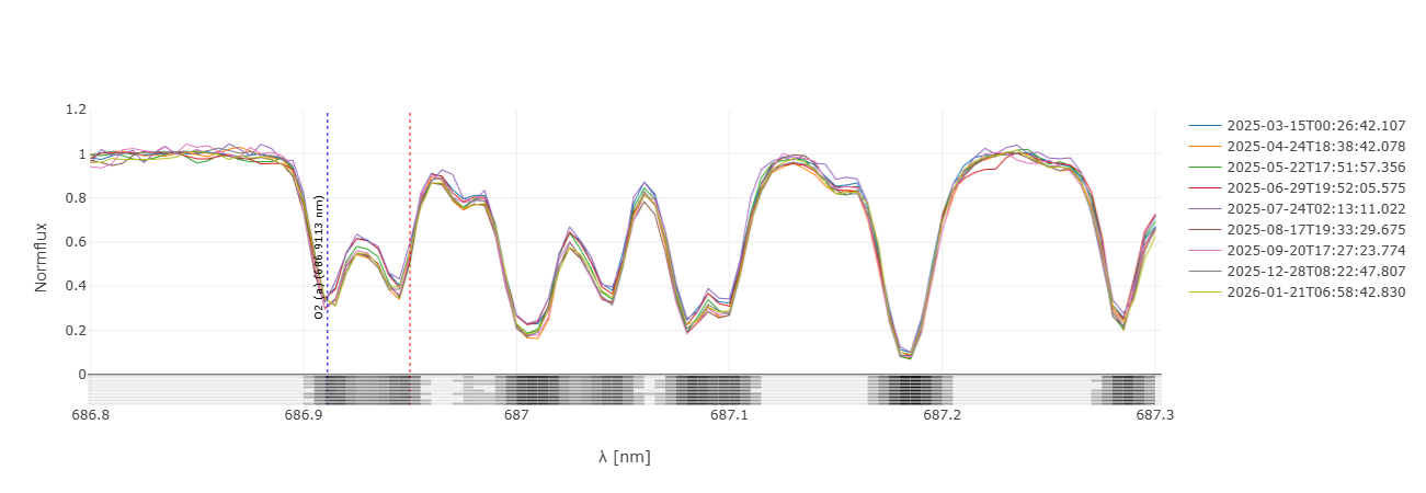
These telluric lines (from the Latin tellus, "earth") are a useful references when studying stellar spectra.
The difference between spectral classes O, A, F, and M is evident in the example of the Mg triplet. The quality of the NRES spectra is demonstrated by a comparison of Mintaka O9 (blue), Vega A0 (orange), Procyon F5 (green), and Antares M1 (red).
This GIF animation can be created from NRES files with just a few clicks, offering students a quick, engaging overview.
The examination of additional prominent lines, as well as the width of these lines, allows for the relatively precise classification of unknown stars into spectral classes.
Mizar A (Zeta Ursae Majoris) provides a good example of a spectroscopic binary system.
As the two stars orbit each other, the Hβ line sometimes splits into two separate lines. This happens because the stars are moving at different speeds toward or away from Earth::
The same effect can be seen in all stellar spectral lines, while the telluric lines from Earth's atmosphere remain unchanged (see Example 1b).
Deneb (Alpha Cygni) is a very large, luminous A2 Ia star that occasionally sheds some of its outer hydrogen-rich gas into space.
This expanding hydrogen envelope is stimulated to glow by the hot star. When we view this glowing gas against the dark background of space, it appears as a bright emission line. Because some of the gas is moving away from Earth, this emission line is shifted toward longer wavelengths (redshift).
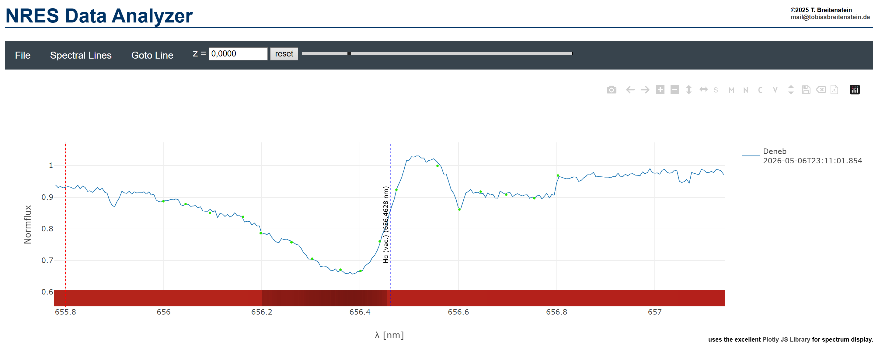
Some of the expanding gas also lies directly between Earth and the star. Although this gas also glows, it absorbs part of the star's light at specific wavelengths. Because the star is much brighter than the surrounding gas, this absorption appears as a dark absorption line in the spectrum. Since this foreground gas is moving toward Earth, the absorption line is shifted toward shorter wavelengths (blueshift).
By measuring these shifts over time, students can study Deneb's outbursts and determine how fast the ejected gas is moving.
VV Cephei is a variable binary star system and is classified as an eclipsing variable. It consists of a red supergiant (VV Cephei A) and a smaller, hotter blue companion (VV Cephei B).
The red supergiant is in a late, unstable stage and has expanded to an enormous size. Because the two stars orbit so close together, the red supergiant exceeds its Roche limit - the point at which a star can no longer hold on to all of its outer gas.
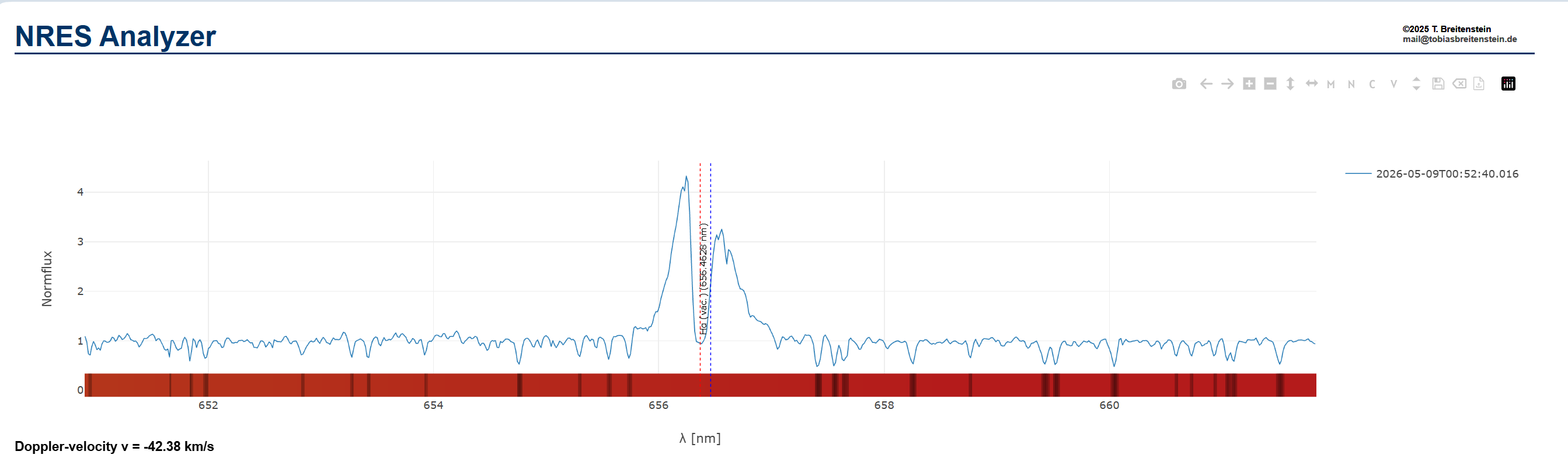
As a result, matter flows onto its smaller, blue companion, forming a rotating disk of material called an accretion disk. This hot accretion disk glows brightly and produces strong Hα emission lines in the NRES spectrum.
The portion of the disk moving away from Earth is redshifted, while the portion moving toward Earth is blueshifted. Near the center of the profile, some of the light from the blue star is absorbed by hydrogen within the disk, producing an absorption feature.
The NRES spectra can also be used for more detailed investigations suitable for research papers or advanced astronomy courses.
The diagram of the spectroscopic binaries Mizar A (Zeta Ursae Majoris) shows not only the splitting of the Hβ line, but rather the astonishing density of the measured values.
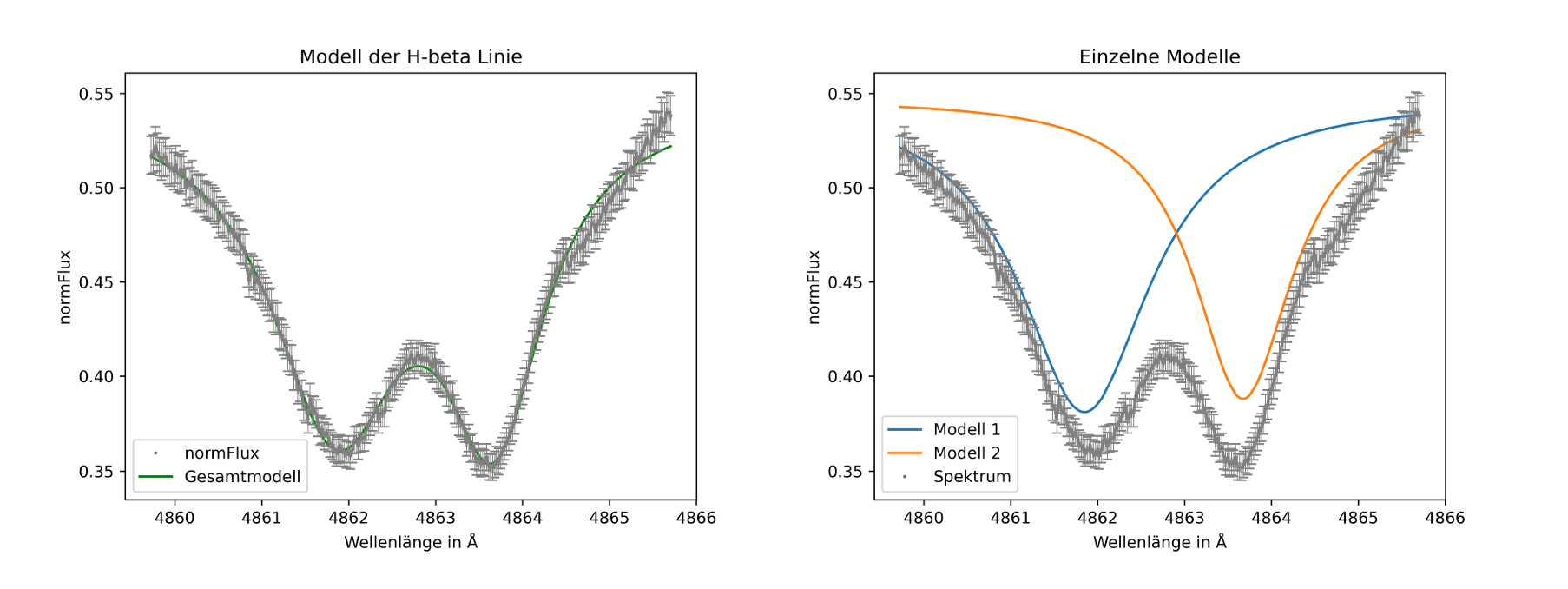
With proper fitting, the radial velocities of both components can be determined with an accuracy of approximately 0.3 km/s. This allows students to move beyond demonstrations and carry out their own scientific investigations using authentic research data.